There are numerous publicly available Resource Description Framework (RDF) datasets that cover a wide range of fields, including geography, life sciences, cultural heritage, and government data. Many of these public datasets can be linked together by loading them into an RDF-compatible database. For example:
DBPedia – An RDF representation of the structured data from Wikipedia
YAGO – A huge multilingual RDF knowledge base, derived from other datasets, including Wikipedia, WordNet, and GeoNames, which contains over 90 million statements about the real world
European Data Portal – Public datasets published by different institutions across the European Union, many of which are in RDF format
RDF is a framework for representing information about resources in a graph form. Unlike traditional databases that store data in tables, RDF structures data as statements of fact called triples, consisting of a subject, predicate, and object. This simple yet powerful model allows for the creation of intricate networks of data.
An example of a triple could be:
<:Kevin> <:worksFor> <:Amazon>
This single statement can evolve into a graph by adding more statements that relate to the first statement:
From this simple RDF graph, we can compute facts that weren’t explicitly stated by following the relationships. For example, Sophie and Kevin live in Seattle, and Sophie works for Amazon.
Because of this simple, natural way for recording data, RDF is inherently interoperable. It’s straightforward to add more statements that talk about the same concepts, and then you have a graph. RDF graph practitioners use this mechanism to link their own data to multiple publicly available RDF datasets. These landscapes of data are known as linked data.
SPARQL is the standard query language for RDF databases. Although powerful, SPARQL is sometimes criticized for missing some useful features, such as pathfinding.
openCypher is a popular graph query language (originally designed for labeled-property graphs, a different graph model from RDF) that enables intuitive and expressive querying, including pathfinding and pattern matching.
In this post, we demonstrate how to build knowledge graphs with RDF linked data and openCypher using Amazon Neptune Analytics.
Amazon Neptune Analytics is a memory-optimized graph database engine for analytics that supports running openCypher queries on RDF data. With Neptune Analytics, you can load massive RDF graphs in seconds and use all the features of openCypher, such as pathfinding, on your RDF datasets.
Solution overview
To perform the solution, we create a Neptune Analytics graph using an import task, which loads the first dataset on creation, then we load a second dataset using batch load. Then we run queries and graph algorithms in Neptune graph notebooks using openCypher.
The solution uses data from the following sources:
Air Routes, an RDF graph that describes airports, airlines, and the routes that airlines use to travel around the globe. The data originates from the OpenFlights Airports Database.
GeoNames, a public RDF geographical database that covers over 11 million place names of different types, ranging from countries and continents to roads, streams, and even some buildings. We use a subset that includes cities, countries, and their metadata.
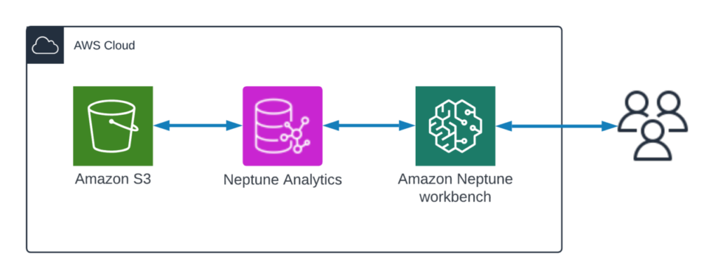
The following diagram illustrates the solution architecture.
The solution uses the following services:
Neptune Analytics – Neptune Analytics is an analytics database engine that can quickly analyze large amounts of graph data in memory.
Amazon SageMaker – We run the Neptune workbench in a Jupyter or JupyterLab notebook on SageMaker. The Neptune graph notebook offers an interactive development environment (IDE) for building graph applications.
Amazon Simple Storage Service (Amazon S3) – Amazon S3 is an object storage service offering industry-leading scalability, data availability, security, and performance.
There are five high-level steps to complete:
Create a Neptune Analytics graph, initializing it with Air Routes RDF data
Create a Neptune graph notebook and connect it to the new graph
Run openCypher queries over the new Air Routes graph in the notebook
Batch load GeoNames RDF data from Amazon S3 into Neptune Analytics using the Neptune.load command
Run openCypher queries and Neptune graph algorithms on the linked RDF data from both sources in the notebook
Prerequisites
You should have completed all the prerequisites to access AWS services with the AWS Command Line Interface (AWS CLI) and the AWS Management Console, with permissions to create resources in Neptune, Amazon S3, SageMaker, and related services.
No further knowledge of the tools and technologies in this post is needed to follow this walkthrough, but a basic understanding of the following is advised:
SPARQL and RDF
openCypher
Amazon S3
Linked data
Customers are responsible for the costs of running the solution. For help with estimating costs, refer to the AWS Pricing Calculator.
Create a Neptune Analytics graph with the AWS CLI
Complete the following steps to create a Neptune Analytics graph:
Create an AWS Identity and Access Management (IAM) role with Amazon S3 access. Take note of the new role ARN because you’ll need it in the next step.
Start a task to create a graph using an import from Amazon S3 by entering the following command using the AWS CLI, replacing the values where necessary. This will create the graph endpoint, simultaneously loading the first of the two RDF datasets, Airroutes.
From the response, make a note of the task ID.
Using the task ID, check the progress of the creation process by running the following command.
Repeat until you see the status in the response changed to COMPLETED:
Enter the following command to get a summary of the contents of the graph.
The response contains many details about the graph, including lists of the edge labels (RDF predicates) and node labels (RDF class types). Neptune Analytics recognizes RDF classes as property graph nodeLabels, and RDF predicates as property graph edgeLabels:
The following figure illustrates the Air Routes ontology and schema.
Create a Neptune notebook and connect it to the graph
Complete the following steps:
On the Neptune console, choose Graphs in the navigation pane.
Select the graph identifier of your new graph.
Note the endpoint under Connectivity & Security.
Create a Neptune Analytics notebook using AWS CloudFormation, providing the endpoint from the previous step for GraphEndpoint in the CloudFormation stack details.
On the Neptune console, choose Notebooks in the navigation pane.
Select your new notebook and on the Actions menu, choose Open Jupyter.
Run openCypher queries over the RDF graph
In the Neptune notebook, choose the New menu, then choose Python 3.
Select the notebook name and rename it to oc-over-rdf-blogpost.
List all the RDF classes or LPG label types and count their instances
Create a new cell and insert the following query. This query will find a list of labels and the number of instances for each label in the dataset.
Run the cell and observe the results, as shown in the following screenshot.
This query result shows all of the RDF class types as node labels and a count of the number of instances of each of them.
For reference, the following code is the equivalent query in SPARQL.
Return all the properties for an RDF resource or LPG node
Create a new cell and insert the following query to find the node for London Heathrow Airport.
Run the cell and observe the results.
The result shows the node for London Heathrow Airport, its labels, and properties.
For reference, the following code is the equivalent query in SPARQL.
Explore the Air Routes RDF graph using openCypher
We have created a notebook with many example openCypher queries to help you explore running openCypher queries over the Air Routes RDF graph.
In the Neptune workbench, choose the Jupyter logo to the root folder. To open the 01-Air-Routes notebook, navigate to Neptune/02-Neptune-Analytics/04-OpenCypher-Over-RDF/01-Air-Routes.ipynb.
If you have been following this post, you already loaded the Air Routes and GeoNames RDF graphs, so you can ignore the load steps.
Walk through the rest of the notebook, running queries and reviewing the responses and visual network graph diagrams.
Load GeoNames RDF data into the graph
Load another RDF graph, which is a subset of GeoNames, including cities and countries to create a graph of linked data.
In the Neptune workbench, choose the Jupyter logo to navigate to the root folder and select the oc-over-rdf-blogpost notebook.
Create a new cell and run the following query to load the GeoNames graph.
You can now run openCypher queries that return linked data from the Air Routes and GeoNames graphs.
Run the first cell again to return a list of labels and the number of instances for each label in the dataset.
The result of the query now contains GeoNames and Air Routes data, as shown in the following table.
Label
Count
<http://neptune.aws.com/ontology/airroutes/Route>
37505
<http://www.geonames.org/ontology#Feature>
28696
<http://schema.org/City>
28444
<http://neptune.aws.com/ontology/airroutes/Airport>
7811
<http://neptune.aws.com/ontology/airroutes/City>
6955
<http://neptune.aws.com/ontology/airroutes/Airline>
6162
<https://www.geonames.org/ontology#Code>
690
<http://www.w3.org/2002/07/owl#Restriction>
636
<http://neptune.aws.com/ontology/airroutes/Country>
356
<http://schema.org/Country>
252
Run a linked data query
Create a new cell and run the following query to find countries from both datasets that have the same ISO country code.
The result shows countries from both datasets linked by ISO country code, as shown in the following table.
#
gn_country.gn::name
ar_country.rdfs::label
1
Saudi Arabia
Saudi Arabia
2
Mayotte
Mayotte
3
Mozambique
Mozambique
4
Madagascar
Madagascar
5
Afghanistan
Afghanistan
6
Pakistan
Pakistan
7
Bangladesh
Bangladesh
8
Turkmenistan
Turkmenistan
9
Tajikistan
Tajikistan
10
Sri Lanka
Sri Lanka
Explore the Air Routes GeoNames RDF graph using openCypher
In the Neptune workbench, choose the Jupyter logo to return to the root folder. To open the 02-Air-Routes-GeoNames notebook, navigate to Neptune/02-Neptune-Analytics/04-OpenCypher-Over-RDF/02-Air-Routes-GeoNames.ipynb.
Step through the 02-Air-Routes-GeoNames notebook to learn how to create more complex queries that span the two datasets.
Clean up
To clean up the resources you created, complete the following steps:
To delete the Neptune Analytics graph, in the AWS CLI, remove delete graph protection using the update-graph command:
Then run the delete-graph command:aws neptune-graph delete-graph –graph-id <graph ID>
On the AWS CloudFormation console, choose Stacks in the navigation pane.
Select the stack that you used to create the Neptune Analytics notebook.
On the Actions menu, choose Delete stack.
Confirm the deletion when prompted.
Summary
In this post, we showed you how to load an RDF dataset into a Neptune Analytics graph using the AWS CLI, and how to query that data with openCypher. We then showed how to load a public dataset and query both datasets in a linked data graph.
Now you can load RDF graphs into Neptune Analytics, link them to your own data, and even run graph algorithms over all the linked data together. There are many large, public RDF datasets available, and you can load massive RDF datasets into Neptune Analytics in seconds.
Visit the openCypher over RDF demo application to see an example architecture, run analytics queries, and browse a network graph visualization that uses the same Air Routes RDF model.
About the Author
Charles Ivie is a Senior Graph Architect with the Amazon Neptune team at AWS. As a highly respected expert within the knowledge graph community, he has been designing, leading, and implementing graph solutions for over 15 years.
Source: Read More

